Module 1: Data Preprocessing
1.1 What is Preprocessing?
Raw point clouds from LiDAR or RGB‑D cameras often contain millions of points. Processing such large clouds directly is too slow and consumes too much memory, especially on embedded systems or in real‑time applications. Preprocessing reduces the number of points while preserving the important geometric structures.
The most common preprocessing operation is downsampling – reducing the point count. Different downsampling methods have different trade‑offs between speed, geometric preservation, and uniformity of the output cloud. In this module, we introduce four widely used methods: voxel downsampling, uniform downsampling, random downsampling, and farthest point sampling (FPS).
1.2 Voxel Downsampling

Voxelization divides 3D space into small cubes (voxels) of edge length \(v\). For every occupied voxel, we compute the centroid (average position) of its points \(P_v = \{p_1,\dots,p_m\}\):
This acts as a low-pass filter, averaging out sensor noise and producing a spatially uniform distribution. It is the industry standard for preparing data before feature extraction, though it may smooth over tiny details if the voxel size is too large.
1.3 Uniform Downsampling
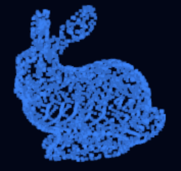
This method treats the point cloud as a linear array and simply selects every \(k\)-th point: \(\{p_k,p_{2k},p_{3k},\dots\}\). While extremely fast (\(O(N)\) complexity) with no spatial search required, it is highly sensitive to the acquisition order. If the sensor follows a periodic scanning pattern, this can cause spatial aliasing, potentially missing entire geometric features.
1.4 Random Downsampling
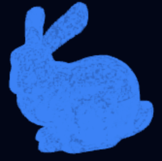
Given a retention ratio \(r\), each point is kept independently based on a random variable \(U_i \sim [0,1]\). The indicator function is:
It is a linear-time method that requires no complex data structures. However, it is non-deterministic and can distort local density, making it best suited for quick previews rather than high-precision tasks.
1.5 Farthest Point Sampling (FPS)
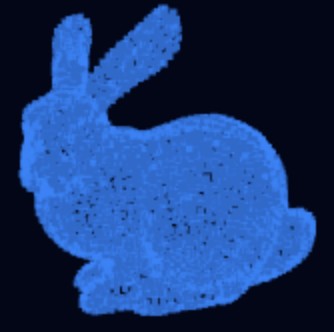
FPS is a greedy algorithm that starts from a random point and iteratively picks the point \(p_k\) that is farthest from the already selected set \(S_{k-1}\):
FPS ensures optimal geometric coverage, making it excellent for preserving boundaries and corners. While slower than other methods (\(O(N\cdot M)\)), it is the preferred choice for deep learning architectures to ensure representative sampling.
1.6 Comparison and Practical Advice
| Method | Speed | Geometric Preservation | Uniformity | Noise Smoothing |
|---|---|---|---|---|
| Voxel | Medium | Good | High | Yes |
| Uniform | Very fast | Poor | Depends on order | No |
| Random | Very fast | Poor | Low | No |
| FPS | Slow | Excellent | High | No |
Recommendations for beginners:
- Start with voxel downsampling. It is the safest and most widely used choice.
- Use random or uniform only when you need a very quick reduction and can tolerate some loss of structure.
- Use FPS when you need the best possible shape preservation and have enough computational power.
1.7 Operating instructions
Select your 3D models and configure environmental variables. This module allows you to evaluate how different data qualities affect the performance and robustness of registration algorithms. Additionally, noise injection adjustments can be applied to evaluate the algorithm's robustness.
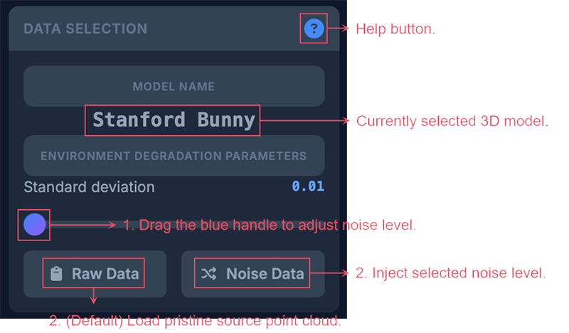
| Parameter | Meaning | Adjustment Guide |
|---|---|---|
| Standard deviation (m) | Amount of Gaussian noise added to point positions. | Increase to simulate low-quality sensors; decrease for high-precision scenarios. |
| Raw Data | Original clean point cloud without synthetic degradation | Use as baseline or ground truth for comparison. |
| Noise Data | Raw data + Gaussian noise. | Use to test robustness of registration algorithms. |
Raw sensor data often contains millions of points, exceeding hardware memory and processing limits. The objective is to reduce data volume through spatial downsampling while preserving the essential geometric structure and topology of the scene.
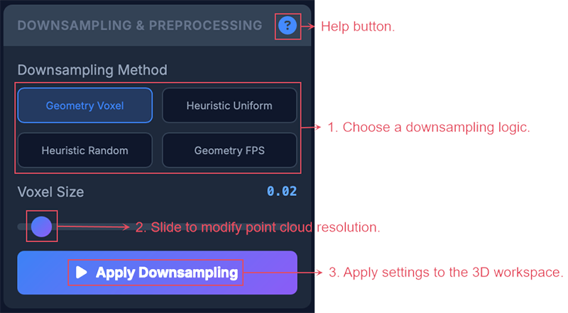
| Parameter | Meaning | Adjustment Guide |
|---|---|---|
| Geometry Voxel | Downsample by averaging points inside fixed 3D cubes | Good for uniform density; keeps geometry. Adjust voxel size: smaller → more points & slower; larger → faster but coarser. |
| Heuristic Uniform | Keep points at roughly uniform spatial intervals. | Use when you want even distribution without voxel bias. |
| Heuristic Random | Randomly select subset of points. | Fastest but least repeatable; good for very large datasets where speed > accuracy. |
| Geometry FPS | Select points farthest from already selected ones. | Best for preserving coverage/extremities. Slower than random but better geometric representation. |